Descriptive statistics provide summaries of quantitative data, which can include quantified qualitative data. They are intended to describe the data as they are rather than draw conclusions beyond your sample of participants. Thus, they are used for descriptive research questions. Inferential statistics are needed to address relational or causal research questions.

For example, if you had two groups with average test scores of 85 and 90, descriptive statistics would say that one group scored higher than the other. This difference does not necessarily mean that there is a statistically significant difference between the two groups. To draw that conclusion (i.e., that the difference is likely not due to chance), you would need to compare this difference to the error within groups. With descriptive statistics, you could not claim that you’d expect to see the same difference in other classes.

Many people learned the basics of descriptive statistics early in school, so I’ll only recap the types of descriptive statistics before talking about features relevant to education research. There are three types of descriptive statistics: 1) central tendency – mean, median, and mode, 2) frequency – percentage, counts, and 3) variability – standard deviation, quartiles, range, kurtosis, and skewness.

Representing Groups of Individuals

In quantitative educational research, we often compare a group of students with one or more features (e.g., taking a class or receiving an intervention) to a group without those features. In this type of paradigm, the unit of interest is a group’s score rather than an individual’s score, and you can represent the group with a measure of central tendency. The mean (M), or average score, is typically the most appropriate descriptive statistic to represent a group with a normal distribution.

If you have skewed data, then you might consider using the median, or middle score, instead. If you are comparing students along a continuum (e.g., prior experience), then measures of frequency and variability are likely more valuable than a measure of central tendency.

Representing Differences Within and Between Groups

Besides the mean, we typically also want to know how homogenous a group’s scores are. For example, a group that has an average test score of 85 with all individual scores in the 80s is more homogenous than a group that has an average test score of 85 with individual scores between 70 and 100. Standard deviation (SD) is a unit that allows you to describe how dispersed scores in a group are. In the test score example, the first group’s scores are closer together, so the standard deviation would be lower than in the second group.

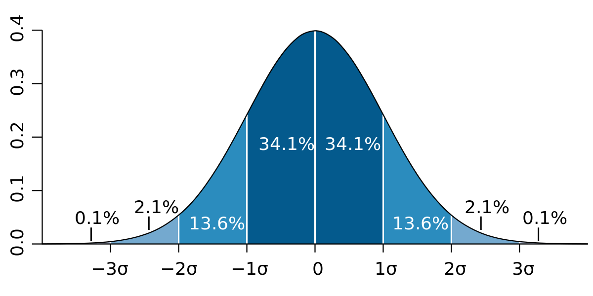
If data follow a normal distribution, there are many interesting things we can learn from standard deviation. For example, about 68% of scores will fall within one standard deviation of the mean (i.e., -1 SD to +1 SD), 95% of scores within two standard deviations (i.e., -2 SD to +2 SD), and 99% within three standard deviations (i.e., -3 SD to +3 SD). For example, if a normally distributed group has a mean of 85 and a standard deviation of 2, then 68% of scores will be between 83 and 87, 95% of scores between 81 and 89, and 99% of scores between 79 and 91.

Interpreting Descriptive Statistics

We can also use these percentages to understand the differences between groups. For example, let’s say we’re comparing two groups — an intervention and a control group — and the intervention group is 1 SD above the control group. The average person in the intervention group will score higher than 84% of the people in the control group (i.e., 50% at the mean + 34.1% in the first standard deviation). Conversely, the average person in the control group will score lower than 16% of the people in the intervention group.

The clustering of scores around the mean is why having 1 SD between groups is such a large difference. Using the same comparison, a 0.2 SD between groups would correspond to the average person in the intervention group scoring higher than 58% of the control group, a 0.5 SD between groups would correspond to 69%, and a 0.8 SD between groups would correspond to 79%. This is why even small effect sizes, explained in a later post, can be meaningful.

To view more posts about research design, see a list of topics on the Research Design: Series Introduction.