The purpose of inferential statistics is to determine if the features of a sample (e.g., participants in a study) are representative of a population (i.e., all people belonging to a group). For example, the question “Do first-generation college students study more than other students?” must be answered with inferential statistics unless you can collect data from all college students. Thus, inferential statistics allow you to make some generalizations about your findings beyond your sample, and they are used to answer relational and causal research questions. The posts on inferential stats will cover many topics (at least two semesters of stats classes), so to break it up, this post will focus on only relational questions.

Correlational Analyses

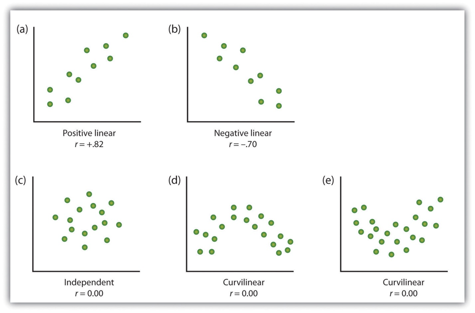
For relational questions, you are trying to determine the type of relationship between two variables. A positive relationship suggests that as the value of a variable increases or decreases, the value of the other variable also increases or decreases, respectively. For example, as attendance in class increases, scores on a test increase as well. A negative relationship is the opposite and suggests that as the value of a variable increases or decreases, the value of the other variable will do the opposite. For example, as absences from class increase, scores on a test decrease.

These are both types of linear relationships; the relationship is constant across different levels of the variables. There are also curvilinear relationships in which the relationship changes across different levels of the variables, often called a U-shaped curve. For example, as students’ level of stress about an exam increases, their scores might increase up to a point, but at that point, excess stress might negatively relate to test scores. These types of curvilinear relationships cannot be analyzed with correlations. A scatterplot of the variables will show you the type of relationship that you have. The images below provide examples of what each type of relationship looks like in a scatterplot. Your data likely won’t be as neat, so you’ll need to ignore the random points that don’t follow the general relationship.

You should choose your correlational analysis based on features of your data, specifically whether your variables are continuous (i.e., interval or ratio) or discrete (i.e., nominal or ordinal). Discrete variables that are dichotomous, a variable that has two values (e.g., yes or no, introvert or extravert), can be either truly dichotomous or artificially dichotomous. Truly dichotomous variables have discrete values (e.g., a participant either has or has not taken Calculus before). Artificially dichotomous variables are continuous variables that the experimenter has split into discrete groups. For example, participants can take a personality test that will rank their personality on a spectrum from introverted to extroverted, and the experimenter could pick a score and classify all participants below that score as introverted and those above the score as extroverted. Artificially dichotomizing variables this way is generally not recommended, but there are rare cases when it’s appropriate.

• If both variables are continuous, use Pearson’s r correlation (this is most common and is typically the default option for analysis software).
• If one variable is truly dichotomous and the other is continuous, use point biserial correlation.
• If one variable is artificially dichotomous and the other is continuous, use biserial correlation.
• If you have discrete data with more than two values (polytomized instead of dichotomized), then you’ll have to use some of the more obscure tests, such as tetrachoric, polychoric, polyserial, Spearman’s rho, or Kendall’s Tau-B.
• If both variables are dichotomous (true or not), you cannot use correlation. Consider descriptive statistics or perhaps Chi-square.

Interpreting Results

The results of a correlational analysis, or correlation coefficient, will be an r (if Pearson’s) value between -1 and 1. Negative numbers indicate a negative relationship, and positive numbers indicate a positive relationship. The closer the number is to 1, the stronger the relationship between variables. The closer the number is to 0, the weaker the relationship between variables. The strength of the relationship indicates how accurately you can predict one variable if you have a value for the other variable. In strong relationships, having values for both variables is somewhat redundant. In weak relationships, the value of one variable provides little information about the other.

**Note** Many people misinterpret the strength of the relationship as the slope of the relationship, but a correlation coefficient of 1 does not mean that the variables have a 1-to-1 relationship.

Below is a table for the heuristic cut-offs (Cohen, 1988) to describe strengths of relationships, but the meaningfulness of the strength of a relationship depends largely on the variables that you are correlating. In educational research especially, correlation coefficients tend to be low because of the large variability in learners’ prior knowledge, level of motivation, etc.

Value of correlation coefficient	Strength of relationship
r >0.5 or <-0.5	Strong
r = |0.5| to |0.3|	Moderate
r = |0.3| to |0.1|	Weak
r = -0.1 to 0.1	No relationship

Correlation vs. Causation

For correlational analyses, a relationship should not be misinterpreted as causal for two reasons: the third variable problem and the directionality problem. The third variable problem states that a third variable, separate from those in the correlation, might be mediating the relationship. In the stress and test score example from earlier, it is unlikely that stress primarily causes better test scores. More likely, stress causes more or better studying, which causes better test scores. The directionality problem states that it is unclear from a correlational analysis which variable is causing which. In the stress and test score example, it is unclear whether high stress hurts test scores or poor test scores cause high stress.

The next post will discuss inferential statistics for causal research questions. To view more posts about research design, see a list of topics on the Research Design: Series Introduction.